In the "Key concepts" section, we explain the basic concepts of trading that are necessary, above all, for understanding our strategy articles. The aim is to introduce beginners to complex strategies and at the same time give advanced traders the opportunity to refresh their basic knowledge.
Bollinger Bands
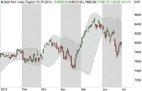
The Bollinger Bands can be used to determine the level of prices relative to previous values. The bands are calculated on the basis of a moving average (GD), in the default setting over 20 periods. The upper Bollinger band is calculated from the GD plus twice the standard deviation of the prices (as a measure of volatility). The lower band is calculated analogously from the GD minus the double standard deviation. If the bands are close together, there is a period of low volatility. If they are far apart, there is a period of high volatility.
Image 1: Bollinger bands
The bands describe a course channel for the prices, which corresponds to two standard deviations in each case. Statistically speaking, on average around 95 percent of all prices should lie within the bands.

Dow theory
The Dow theory was developed by the American economist Charles Henry Dow. It represents the theoretical background for trend lines and trend channels. Dow defined a trend as a market movement clearly pointing in a certain direction. Basically, there are three possibilities: Upward trend, Downward trend and Sideward trend. Depending on the time frame, each index or security can show several - possibly opposing - trends. The long-term trend is referred to as the primary trend; it can last for a year or longer. Within the primary trend, secondary trends can occur for which a duration of up to three months is usually estimated. Tertiary trends are more short-term and last from one week to a maximum of one month.
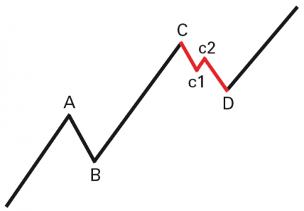
Image 2: Dow Theory
Within the primary trend (A, B, C, D) secondary trends (c1, c2) may occur.
Fibonacci retracements
The Fibonacci numbers are an infinite sequence. A Fibonacci number is calculated by adding the two preceding numbers. The sequence starts with 0 and 1. All following numbers result automatically: 2, 3, 5, 8, 13 and so on. Fibonacci numbers and ratios often occur in nature; their application in technical analysis also transfers this to the financial markets. Fibonacci retracements - in the sense of returns or corrections - are determined by first searching for two extreme points in the chart, a low and a high. This distance corresponds to 100 percent of the movement. Based on this, the retracements are different correction levels such as 38.2, 50 or 61.8 percent. These values result from the formation of different quotients in the Fibonacci number sequence.
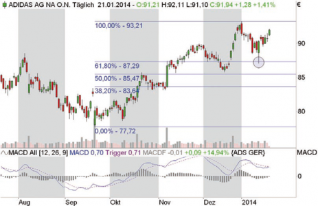
Image 3: Fibonacci retracement and MACD
Shown are the MACD and a 38.2% Fibonacci retracement at adidas. From the price increase in mid-September to the end of December 2013, the share corrected intraday by 38.2 percent in January, almost exactly to the cent, closing the remaining gap in mid-December at the same time and then rising again. About the MACD: The histogram describes the difference between the blue MACD and the violet signal line.
Moving average
The simplest way to calculate an average is known as the arithmetic mean. The calculation is simple: you divide the sum of the prices or indicator values of the calculation period by the number of trading days contained. In technical analysis, this continuously calculated value is referred to as the Moving Average (GD). The GD is already known from times when traders drew their charts by hand on graph paper and carried out simple calculations with a pencil. The simplicity of the calculation has nothing to do with the quality and benefit of the result. The simple GD is used today just as often as other types of GDs that are more complicated to calculate, such as simply weighted or exponentially weighted GDs. In general, GDs are used as part of trading systems, as signal lines in indicators and to determine trends in stock, future and index charts.
Keltner Channel
The Keltner Channel assumes a moving average of the typical price. The channel limits are adapted to the prevailing fluctuation intensity of the underlying value. Keltner used an average of the daily trading margin, while many software packages use the Average True Range. The bands are calculated by adding or subtracting the ATR weighted by a factor from the GD of the typical price. The Keltner Channel is often used to follow trends, as it is based on a sudden increase in volatility with a new, strong trend movement. Subsequently, the bands are touched, since their calculation is delayed due to the GDs. If the price breaks out of the upper band, it is considered a buy-signal; if it breaks out of the lower band, it is considered a sell-signal. If the multiplier is too large for the ATR, these breakouts occur quite late and much of the trend movement remains unused. Alternatively, a return from outside the bands back into the bands can be used as a trading signal. If the price returns from below into the channel, this is considered a buy-signal, it returns from above as a sell-signal.
Image 4: Keltner Channel
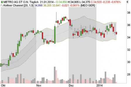
Using the Keltner Channel, it was easy to distinguish between sideways and trend phases at Metro. A sideways phase occurs when the prices move within the bands - in this case the Metro share price since the beginning of December 2013. If the prices close significantly outside the bands, there is a corresponding trend, in this case upwards in October and November 2013.
Moving Average Convergence/Divergence (MACD)
The indicator developed by Gerald Appel and widely used in trading calculates two lines. The faster line (called the MACD line) is the difference between two exponentially smoothed moving averages based on closing prices, usually the last twelve and 26 days or weeks. The slower line (signal line) is usually an exponentially smoothed 9-period average of the MACD line. Most investors trade buy and sell signals resulting from the crossing of the two lines. The difference between the lines can also be displayed in the MACD histogram for better visualization.
Relative Strength Index (RSI)
The Relative Strength Index (RSI) was conceived by Welles Wilder Jr. and presented to the public in his 1978 book "New Concepts in Technical Trading Systems". The RSI, which like the MACD is one of the most widely used technical indicators, is calculated according to the formula:
RSI = 100 - 100 / (1 + RS)
With the RSI, the extent of price losses can be compared with the price gains of the same period. In the formula RS (relative strength) stands for the quotient of the average of the closing prices of x days/weeks with rising prices and the average of the closing prices of x days/weeks with falling prices. Usually 14 days or weeks are used as the value for x. To determine the mean value for the days/weeks with a positive price trend, the total price gains accrued within the 14 days/weeks on days/weeks with rising prices must be added and divided by 14. To calculate the average value for days/weeks with a negative price trend, the total price losses incurred during this period on days/weeks with falling prices must be added up and divided by 14. The relative strength is then calculated by dividing the average price gain by the average price loss. The RS is then inserted into the RSI formula.
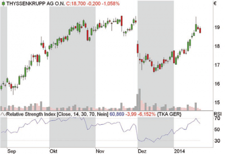
Figure 5: Relative Strength Index (RSI)
Prices above the 70 mark are considered oversold at the RSI, below the 30 mark they are considered oversold.
Source: TRADERS' Mag.